vSAN Slack Space is the free space in the vSAN Datastore reserved for vSAN’s internal operational and rebuild actions such as..
Rebalancing operations and VM snapshots
Component rebuilds – If you have a FTT=1 RAID1 vSAN storage Policy and you decide to change this to a FTT=1 RAID5 storage policy, vSAN will need to use extra space to perform this type of change.
Host maintenance mode data evacuation
VMware used to recommend 25-30% of free space for Slack Space although from 7.0u1 there are a couple of new features under the Reservation and Alerts section of the vSAN Services on a cluster which can be used to control this space. You will hear it called Capacity Reserve to reflect the methodical and improved approach to compute reserve capacity.
Operations reserve
Host rebuild reserve
By default, these features are disabled, meaning all vSAN capacity is available for workloads.
Reserved capacity is not supported on stretched clusters, clusters with fault domains and nested fault domains, ROBO cluster or if the cluster has less than 4 hosts.
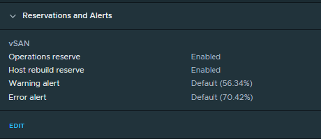
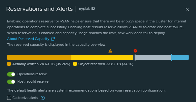
Reservations and Alerts
Enabling Operations Reserve for vSAN ensures that there will be enough space in the cluster for internal operations to complete successfully.
Enabling Host Rebuild Reserve allows vSAN to tolerate one host failure
When reservation is is enabled and capacity usage reaches the limit, new workloads fail to deploy or power on but existing VMs are fine.
Click Edit to view
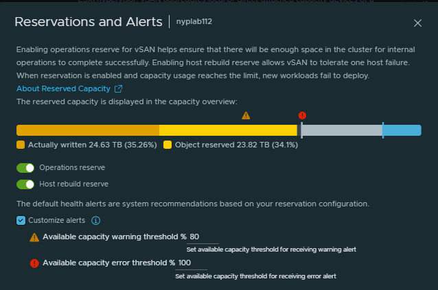
You can customise the thresholds of when to receive warning and error alerts. The threshold percentage is calculated based on available capacity which is the total capacity minus the reserved capacity. If you do not set customised values, vSAN will use the default thresholds to generate alerts.
Operation reserve
This is basically the capacity set aside for vSAN to run it’s internal operations as seen earlier – host maintenance mode data evacuation, component rebuilds, rebalancing operations, and VM snapshots. Activities such as rebuilds and rebalancing can temporarily consume additional raw capacity.
Host rebuild reserve
The first parameter is Host Rebuild Reserve. This reservation is set to one host worth of capacity. This means that if one host in the vSAN cluster fails and no longer contributes storage, there is still sufficient capacity remaining in the cluster to rebuild and re-protect all vSAN objects. This reservation is based on the N+1 host count recommendation. In small clusters, the percentage is high (e.g. 25% in a 4-node cluster), the percentage decreases significantly as the number of hosts in vSAN cluster increases (single digit 8% approx of capacity values for clusters > 12 nodes). For example, a 48-node cluster can improve capacity savings up to 18%, resulting in greater resource optimization at a lower cost.
Unfortunately you cannot simply enable Host rebuild reserve on its own when enabling Operation Reserve. You must enable Operations reserve and then you can choose to enable Host rebuild reserve as well, or leave it disabled. Be aware that the 10% overhead of the Operations threshold is taken into consideration before the Host rebuild reserve is taken into account. For example, in a small 4/6 node vSAN cluster, the 10% Operations Reserve is first calculated and accounted for, before the Host rebuild reserve threshold is taken into account.
Considerations for both Operations reserve and Host rebuild reserve enabled
When you enable Operations reserve with the Host rebuild reserve and a host is put into maintenance mode, the host may not come back online. In this case, vSAN continues to reserve capacity for another host failure. The host failure is in addition to the host that is already in maintenance mode. This might cause the failure of operations if the capacity usage is above the host rebuild threshold
When you enable reserved capacity with the Host rebuild enabled and a host fails, vSAN may not start repairing affected objects until the repair timer expires. During this time vSAN continues to reserve capacity for another host failure. This can cause failure of operations if the capacity usage is above the current host rebuild threshold. After any repairs are complete, you can deactivate the reserved capacity for the host rebuild if the cluster does not have the capacity for another host failure.
Artificial Intelligence (AI) is the branch of computer science focused on creating systems capable of performing tasks that normally require human intelligence. These tasks include things like understanding natural language, recognizing patterns, solving problems, and making decisions.
AI systems use algorithms and large datasets to “learn” from data patterns, which is often referred to as machine learning. This allows them to improve their performance over time. Applications of AI range widely, from healthcare diagnostics and financial modeling to self-driving cars and language translation. There are different types of AI:
Narrow AI (or Weak AI): Designed to perform a specific task, like voice assistants (e.g., Siri), image recognition, or playing chess.
Broad AI Broad AI is a midpoint between Narrow and General AI. Rather than being limited to a single task, Broad AI systems are more versatile and can handle a wider range of related tasks. Broad AI is focused on integrating AI within a specific business process where companies need business- and enterprise-specific knowledge and data to train this type of system. Newer Broad AI systems predict global weather, trace pandemics, and help businesses predict future trends.
General AI (or Strong AI): Hypothetical AI that could understand, learn, and apply knowledge in any domain, similar to human intelligence. This level of AI doesn’t yet exist.
Artificial Superintelligence (ASI): A potential future stage where AI surpasses human intelligence in all fields 😮
Augmented Intelligence
There is also the term augmented intelligence. AI and augmented intelligence share the same objective, but have different approaches. Augmentedintelligence tries to help humans with tasks that are not practical to do. For example, in healthcare, augmented intelligence systems assist doctors by analyzing medical data, such as imaging scans, lab results, and patient histories, to identify potential diagnoses. For instance, IBM Watson Health provides doctors with insights based on large volumes of medical data, suggesting possible diagnoses and treatment options. The doctor then uses this information, combined with their own expertise, to make the final decision. However, artificial intelligence has the aim of simulating human thinking and processes.
What does AI do?
AI services can ingest huge amounts of data. They can apply mathematical calculations in order to analyze data, sorting and organizing it in ways that would have been considered impossible only a few years ago. AI services can use their data analysis to make predictions. They can, in effect, say, “Based on this information, a certain thing will probably happen.”
Some of the most commonly cited benefits include:
Automation of repetitive tasks.
More and faster insight from data.
Enhanced decision-making.
Fewer human errors.
24×7 availability.
Reduced physical risks.
The history of AI
The Eras
How do we understand the meaning that’s hidden in large amounts of data. Information can be difficult to extract and analyse from a very large amount of data. Because it’s hard to see without help, scientists call this dark data. It’s information without a structure. During the mid-1800s in England, Charles Babbage and Ada Lovelace designed what they called a “difference engine” designed to handle complex calculations using logarithms and trigonometry. It wasn’t finished but if they had completed it, the difference engine might have helped the English Navy build tables of ocean tides and depth soundings to assist sailors. In the early 1900s, companies like IBM were using machines to tabulate and analyze the census numbers for entire national populations. They found patterns and structure within the data which had useful meaning beyond simple numbers. These machines uncovered ways that different groups within the population moved and settled, earned a living, or experienced health problems, information that helped governments better understand and serve them. By the early 1900s, companies like IBM were using machines to tabulate and analyze the census numbers for entire national populations. They didn’t just count people. They found patterns and structure within the data—useful meaning beyond mere numbers. These machines uncovered ways that different groups within the population moved and settled, earned a living, or experienced health problems—information that helped governments better understand and serve them. Researchers call these centuries the Era of Tabulation, a time when machines helped humans sort data into structures to reveal its secrets.
During World War II, a groundbreaking approach took shape to handling vast amounts of untapped information; what we now refer to as “dark data”, marking the beginning of the Programming Era. Scientists developed electronic computers capable of processing multiple types of instructions, or “programs.” Among the first was the Electronic Numerical Integrator and Computer (ENIAC), built at the University of Pennsylvania. ENIAC wasn’t limited to a single function; it could perform a range of calculations. It not only generated artillery firing tables for the U.S. Army but also undertook classified work to explore the feasibility of thermonuclear weapons. The Programming Era was a revolution in itself. Programmable computers guided astronauts from Earth to the moon and were reprogrammed during Apollo 13’s troubled mission to bring its astronauts safely back to Earth.Researchers call these centuries The Programming Era, a much more advanced era of AI
In the early summer of 1956, a pioneering group of researchers led by John McCarthy and Marvin Minsky gathered at Dartmouth College in New Hampshire, one of the oldest institutions in the United States. There, they sparked a scientific revolution by coining the term “artificial intelligence.” These researchers envisioned that “every aspect of learning or any other feature of intelligence” could be so precisely defined that a machine could be built to replicate it. With this vision of “artificial intelligence,” they secured substantial funding to pursue it, aiming to achieve their goals within 20 years. Over the next two decades, they made remarkable strides, creating machines that could prove geometry theorems, engage in basic English dialogue, and solve algebraic word problems. For a time, AI became one of the most thrilling and promising fields in computer science. However limited computing power and limited information storage restricted the progress of AI at the time. Researchers call this The Era of AI. It took about a decade for technology and AI theory to catch up. Today, AI has proven its ability in fields ranging from cancer research and big data analysis to defense systems and energy production.
Types of data
Data is raw information. Data might be facts, statistics, opinions, or any kind of content that is recorded in some format.
Data can be organized into the following three types.
Structured data is typically categorized as quantitative data and is highly organized. Structured data is information that can be organized in rows and columns. Similar to what we see in spreadsheets, like Google Sheets or Microsoft Excel. Examples of structured data includes names, dates, addresses, credit card numbers, employee number
Unstructured data,also known as dark data, is typically categorized as qualitativedata. It cannot be processed and analyzed by conventional data tools and methods. Unstructured data lacks any built-in organization, or structure. Examples of unstructured data include images, texts, customer comments, medical records, and even song lyrics.
Semi-structured data is the “bridge” between structured and unstructured data. It doesn’t have a predefined data model. It combines features of both structured data and unstructured data. It’s more complex than structured data, yet easier to store than unstructured data. Semi-structured data uses metadata to identify specific data characteristics and scale data into records and preset fields. Metadata ultimately enables semi-structured data to be better cataloged, searched, and analyzed than unstructured data.
Experts estimate that roughly 80% of all data generated today is unstructured. This data is highly variable and constantly evolving, making it too complex for conventional computer programs to analyze effectively
AI can start to give us answers on unstructured data! AI uses new kinds of computing—some modeled on the human brain—to rapidly give dark data structure, and from it, make new discoveries. AI can even learn things on its own from the data it manages and teach itself how to make better predictions over time.
As long as AI systems are provided and trained with unbiased data, they can make recommendations that are free of bias. A partnership between humans and machines can lead to sensible decisions.
Can machine learning help us with unstructured data?
If AI is not relying on programming instructions to work with unstructured data, how does AI start to analyse data? Machine learning can analyze dark data far more quickly than a programmable computer can. Think about the problem of finding a route through busy city traffic using a navigation system. It’s a dark data problem because solving it requires working with not only a complicated street map, but also with changing variables like weather, traffic jams, and accidents.
The machine learning process vs AI
The machine learning process has advantages:
It doesn’t need a database of all the possible routes from one location to another. It just needs to know where places are on the map.
It can respond to traffic problems quickly because it doesn’t need to store alternative routes for every possible traffic situation. It notes where slowdowns are and finds a way around them through trial and error.
It can work very quickly. While trying single turns one at a time, it can work through millions of tiny calculations.
Machine learning can predict. As an example, a machine can determine, “Based on traffic currently, this route is likely to be faster than that one.” It knows this because it compared routes as it built them. It can also start to learn and notice that your car was delayed by a temporary detour and adjust its recommendations to help other drivers.
Types of machine learning
There are two other ways to contrast classical and machine learning systems. One is deterministic and the other is probabilistic.
In a deterministic system, there must be a vast, pre-defined network of possible paths—a massive database that the machine uses to make selections. If a particular path reaches the destination, the system marks it as “YES”; if not, it marks it as “NO.” This is binary logic: on or off, yes or no, and it’s the foundation of traditional computer programming. The answer is always definitive—either true or false—without any degree of certainty.
Machine learning, by contrast, operates on probabilities. It doesn’t give a strict “YES” or “NO.” Instead, machine learning is more like an analog process (similar to waves with gradual rises and falls) than a binary one (like sharply defined arrows up or down). Machine learning evaluates each possible route to a destination, factoring in real-time conditions and variables, such as changing traffic patterns. So, a machine learning system won’t say, “This is the fastest route,” but rather, “I am 84% confident that this is the fastest route.” You may have seen this when using maps on your phone where it will give you the option of 2 or more alternative routes.
Three common methods of machine learning
Machine learning solves problems in three ways:
Supervised learning
Unsupervised learning
Reinforcement learning
Supervised learning
Supervised learningis about providing AI with enough examples to make accurate predictions. All supervised learning algorithms need labeled data. Labeled data is data that is grouped into samples that are tagged with one or more labels. In other words, applying supervised learning requires you to tell your model what something is and what features it has.
Unsupervised learning
In unsupervised learning, someone will feeds a machine a large amount of information, asks a question, and then the machine is left to figure out how to answer the question by itself.
For example, the machine might be fed many photos and articles about horses. It will classify and cluster information about all of them. When shown a new photo of a horse, the machine can identify the photo as a horse, with reasonable accuracy. Unsupervised learning occurs when the algorithm is not given a specific “wrong” or “right” outcome. Instead, the algorithm is given unlabeled data.
Unsupervised learning is helpful when you don’t know how to classify data. For example, lets say you work for a distribution company institution and you have a large set of customer financial data. You don’t know what type of groups or categories to organize the data. Here, an unsupervised learning algorithm could find natural groupings of similar customers in a database, and then you could describe and label them. This type of learning has the ability to discover similarities and differences in information, which makes it an ideal solution for exploratory data analysis, cross-selling strategies, customer segmentation, and image recognition.
Reinforcement learning
Reinforcement learning is a machine learning model similar to supervised learning, but the algorithm isn’t trained using sample data. This model learns as it goes by using trial and error. A sequence of successful outcomes is reinforced to develop the best recommendation for a given problem. The foundation of reinforcement learning is rewarding the “right” behavior and punishing the “wrong” behavior.
So what’s the link between AI and Machine Learning?
(Artificial Intelligence) and machine learning (ML) are closely related but are not the same thing. Here’s a breakdown of their relationship and differences:
Artificial Intelligence
Definition: AI is a broad field focused on creating systems or machines that can perform tasks that normally require human intelligence. These tasks can include reasoning, learning, problem-solving, perception, and language understanding.
Scope: AI encompasses various approaches and technologies, including rule-based systems, expert systems, natural language processing, robotics, and, importantly, machine learning.
Goal: The ultimate goal of AI is to create machines that can think and act intelligently, either by mimicking human cognitive functions or by developing entirely new capabilities.
2. Machine Learning
Definition: Machine learning is a subset of AI that specifically involves algorithms and statistical models that allow computers to learn from and make predictions or decisions based on data. Instead of following explicitly programmed instructions, ML models find patterns in data to improve their performance over time.
Scope: ML includes various techniques and algorithms like supervised learning, unsupervised learning, reinforcement learning, neural networks, and deep learning.
Goal: The goal of ML is to develop models that can generalize from data, allowing computers to improve their task performance automatically as they are exposed to more data.
How AI and ML are linked
AI as the Parent Field: AI is the broader field, with ML as one of its key methods for achieving intelligent behavior.
ML as a Tool for AI: ML provides a powerful way to achieve AI by enabling systems to learn from experience and adapt without needing extensive reprogramming.
Types of AI: While ML is currently one of the most effective ways to achieve AI capabilities, other forms of AI (like rule-based systems) do not involve learning from data in the same way.
Summary
AI: The broader goal of creating intelligent systems.
ML: A method within AI that enables systems to learn and improve from data.
In essence, machine learning is one of the main drivers of AI today, especially in areas like computer vision, speech recognition, and natural language processing.
Windows Virtualization-Based Security (VBS) is a security feature in Windows that uses hardware virtualization to create and isolate a secure region of memory from the normal operating system. This secure memory region can be used to host various security solutions, providing protection from vulnerabilities and attacks that could compromise the system.
Key Components and Features of VBS:
Hypervisor-Enforced Code Integrity (HVCI):
Ensures that only signed and verified code can execute in kernel mode.
Uses the hypervisor to enforce code integrity policies, preventing unsigned drivers or system files from being loaded.
Credential Guard:
Isolates and protects credentials such as NTLM hashes and Kerberos tickets using VBS.
Prevents attackers from stealing credentials even if the operating system kernel is compromised.
Device Guard:
Combines HVCI with other features to ensure that the device runs only trusted applications.
Includes Configurable Code Integrity (CCI) and relies on policies that define which code can be trusted.
Secure Kernel Mode:
Runs alongside the normal Windows kernel, but is isolated from it.
Protects key processes and data from being tampered with or read by the normal operating system.
Kernel Data Protection (KDP):
Prevents kernel memory from being tampered with by malicious actors.
Protects non-executable data in the kernel such as data structures, which are vital for the operating system’s security and stability.
How VBS Works:
Hardware Requirements:
Requires modern CPUs with virtualization extensions (such as Intel VT-x or AMD-V).
Requires a system firmware that supports Secure Boot and UEFI.
Typically requires TPM 2.0 for certain features like Credential Guard.
Operational Flow:
At system boot, the Windows hypervisor (Hyper-V) initializes and creates an isolated environment.
The VBS components operate within this environment, isolated from the main operating system and its potential vulnerabilities.
This isolation ensures that even if the main operating system is compromised, the VBS-protected components remain secure.
Benefits of VBS:
Enhanced Security:
Protects against a variety of modern threats, including malware, rootkits, and credential theft.
Provides a stronger security boundary than traditional software-based security measures.
Trustworthy Execution Environment:
Ensures that critical security mechanisms and sensitive data are executed and stored in a protected environment.
Use Cases:
Enterprise Environments:
Provides advanced protection mechanisms for organizations handling sensitive data and requiring stringent security measures.
Helps meet compliance and regulatory requirements by providing enhanced security controls.
Secure Workloads:
Ideal for protecting workloads that handle sensitive or high-value data, such as financial transactions, healthcare records, and government data.
In summary, Windows VBS leverages hardware virtualization to create a secure environment that enhances the security of the operating system, providing robust protection against a wide range of threats and vulnerabilities.
SNMP was created in 1988 (based on Simple Gateway Management Protocol, or SGMP) as a short-term solution and was created to allow devices to exchange information with each other across a network. Since then, SNMP has achieved universal acceptance and become a standard protocol for many applications and device. It is considered “simple” because of its reliance on an unsupervised or connectionless communication link.and was created to allow devices to exchange information with each other across a network
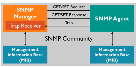
SNMP has a simple architecture based on a client-server model.
The servers, called managers, collect and process information about devices on the network.
The clients, called agents, are any type of device or device component connected to the network. They can include not just computers, but also network switches, phones and printers as an example
SNMP is considered “robust”, because of the independence of the managers from the agents. Because they are typically separate devices, if an agent fails, the manager will continue to function and the opposite is also true.
SNMP is non-proprietary, fully documented, and supported by multiple vendors.
SNMP Ports
SNMP Managers broadcast requests and receive responses on UPD port 161. Traps are sent to UDP port 162.
What versions of SNMP are there?
SNMP Version
Advantages
Disadvantages
SNMP v1
Old version of the protocol now so little advantages compared to v2 and v3
Community string sent in clear text Most community strings set to “public” Only supports 32-bit counters, which is very limiting for today’s networks
SNMP v2c
Supports 64-bit counters
GETBULK command added to request multiple variables from an agent
INFORM” altered the way that “Traps” worked in SNMPv1 making the manager confirm receipt of a message
SNMPv2c brought improvements in areas such as protocol packet types, MIB structure elements, and transport mappings, it still has the same security flaws as its predecessor
SNMPv2 introduced a new security system that, unfortunately, limited the adoption of this new protocol SNMPv2c was developed in response, removing the new security system and reverting to the familiar community approach
SNMPv2c’s simple authentication system and lack of encryption makes networks vulnerable to a wide range of threats.
SNMP v3
SNMPv3 introduces three new elements: SNMP View, SNMP Groups, and SNMP Users. This ensures every interaction with a device on the network is effectively authenticated and encrypted
SNMPv3 also introduced encryption methods such as SHA, MDS and DES to increase security and prevent data tampering and eavesdropping
Encryption systems only work if authentication has been enabled
Multiple variables that need to be configured, including usernames, passwords, authentication protocols, and privacy protocols. Misconfiguration is a serious concern
Not all devices are compatible yet
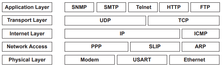
What layer is SNMP found?
SNMP Message Types
SNMP uses six basic messages to communicate between the manager and the agent
GET – The manager can send GET and GET-NEXT messages to the agent requesting information for a specific variable.
GET-NEXT -The SNMP manager sends this message to the agent to get information from the next OID within the MIB tree.
RESPONSE – The agent sends a RESPONSE to the SNMP manager when replying to a GET request. This provides the SNMP manager with the variables that were requested originally.
SET – A SET message allows the manager to request a change be made to a managed object. The object agent will then respond with a GET-RESPONSE message if the change has been made
or an error saying why the change cannot be made.
TRAP – TRAP messages are unique because they are they only message type that is initiated by the agent. TRAP messages are used to inform the manager when an important event happens. This makes TRAPs perfect for reporting alarms to the manager rather than wait for a status request from the manager.
INFORM – Similar to TRAP initiated by the agent, INFORM also includes confirmation from the SNMP manager on receiving a message
MIB
A MIB or Management Information Baseis a formatted ASCII text file that resides within the SNMP manager designed to collect information and organize it into a hierarchical format. It’s essentially a agent-to-manager dictionary of the SNMP language, where every object referred to in an SNMP message is listed and explained. In order for your SNMP manager to understand a device that it’s managing, a MIB must first be loaded (“compiled”).The SNMP manager uses information from the MIB to translate and interpret messages before sending them onwards to the end-use. A long numeric tag or object identifier (OID) is used to distinguish each variable uniquely in the MIB and SNMP messages. MIBs are written in the OID format. In order to read a MIB, you need to load it into an MIB browser, which will make the OID structure visible.
It’s essentially a agent-to-manager dictionary of the SNMP language, where every object referred to in an SNMP message is listed and explained. In order for your SNMP manager to understand a device that it’s managing, a MIB must first be loaded (“compiled”).
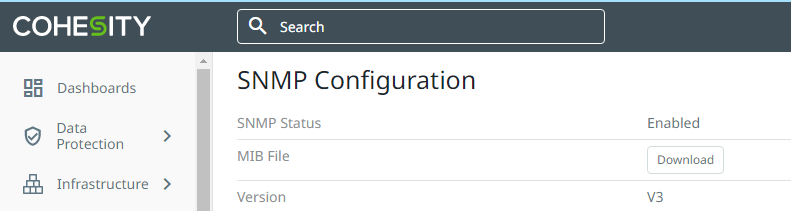
Vendors will make their VIBs available for download when appliances are configured for SNMP. Example from Cohesity below
When an SNMP device sends a Trap or other message, it identifies each data object in the message with a number string called an object identifier (OID). This is great for a computer, but not easily readable for a human being. The MIB provides a text label for each OID. This is similar to DNS servers on the internet that translate numerical IP addresses into domain names that you can understand.
What is an OID?
An OID is an Object Identifier that can be defined by RFC’s. A MIB file is a text file that defines all the OID’s available in that file. If you look at this file it will be hard to understand. You can use a MIB browser which are designed to interpret MIB files and make it easier to understand each OID. Each OID will have a name, a description as well as if SNMP Get’s or Set’s are accepted. Most MIB browsers also have a built in feature to send SNMP Get’s and Set’s. You can search for the specific OID you need.
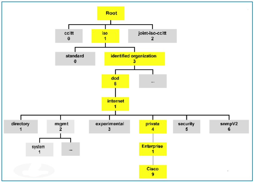
An OID is formatted in a string of numbers as shown below. These numbers each provide you with a piece of corresponding information. Most of the time OIDs will be provided by the vendor you purchased your device from. Example Cisco OID for RAM usage in %
1.3.6.1.4.1.9.9.618.1.8.6.0
Each segment in the number string denotes a different level in the order, starting with one of the two organizations that assign OIDs, all the way down to a unique manufacturer, a unique device, and a unique data object
Every SNMP-enabled network device will have its own MIB table with many different OIDs. There are so many OIDs in most MIBs that it would be next to impossible to record all of the information.
SNMP agents include OIDs with every Trap message they send. This allows the SNMP manager to use the compiled MIB to understand what the agent is saying.
SNMP monitoring tools are designed to take data from MIBs and OIDs to present to you in a format that is easy to understand. Get requests and SNMP traps provide network monitors with raw performance data which is then converted into graphical displays, charts, and graphs. As such, MIBs and OIDs make it possible for you to monitor multiple SNMP-enabled devices from one centralized location.
SNMP v3 Authentication and Encryption
Older versions of SNMP relied on a single unencrypted “community string” for both get requests and traps, making it very insecure on the network (Anyone could ‘snoop’ on the network and detect the unencrypted community strings). The only security options with SNMP v1 and v2c are to either disable it altogether or make sure SNMP enabled devices are ‘read only’ so that if the connection details were obtained by a malicious person, they would only be able to read configuration rather than change device configuration.
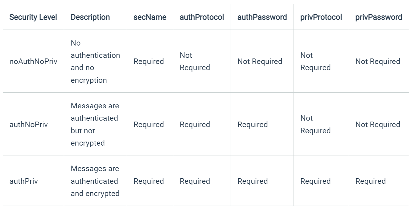
Version 3 uses the same base protocol as version 1 and 2c, but introduces encryption and much improved authentication mechanisms. Depending on how you authorize with the SNMP agent on a device, you may be granted different levels of access.
The security level you use depends on what credentials you must provide to authenticate successfully
Authentication protocols
MD5 and SHA
Privacy protocols
DES and AES
Information on Engine IDs
The protocols used for Authentication are MD5 and SHA ; and for Privacy, DES (Data Encryption Standard) and AES (Advanced Encryption Standard)
Engine IDs
In SNMP (Simple Network Management Protocol), an engine ID is a unique identifier assigned to a SNMP entity. It is a string of octets that identifies a particular SNMP entity within a network or administrative domain.
The engine ID is used in SNMP to distinguish between different SNMP entities and to ensure that SNMP messages are sent to the correct recipient. When an SNMP message is sent, it includes the engine ID of the sending entity, as well as the engine ID of the intended recipient. The engine ID is also used in SNMP to authenticate messages and to ensure that they are generated by a trusted SNMP entity.
There are two types of engine IDs in SNMP:
Local Engine ID – This is the engine ID assigned to the local SNMP entity. It is used to identify the local entity to other SNMP entities in the network.
Remote Engine ID – This is the engine ID assigned to a remote SNMP entity. It is used to identify the remote entity to the local entity when SNMP messages are exchanged between them.
The engine ID is an important aspect of SNMP as it ensures that SNMP messages are sent to the correct recipient and are generated by a trusted SNMP entity.
Context engine
The context engine in SNMP (Simple Network Management Protocol) is responsible for providing context to SNMP messages. SNMP messages are used to manage network devices, and they contain information about the operation to be performed on the network device.
However, SNMP manages a large number of network devices, and it is necessary to identify the specific network device that is being managed. This is where the context engine comes in. The context engine provides the necessary context to SNMP messages to identify the specific network device being managed.
In SNMP, a context is a piece of information that identifies the specific instance of a managed object. Managed objects are objects in the network device that can be managed through SNMP. For example, a managed object could be the interface statistics for a network interface.
The context engine provides the necessary context to SNMP messages in the form of a context identifier (CID). The CID is a string of characters that uniquely identifies the instance of the managed object being managed. The CID is included in the SNMP message, and it allows the SNMP manager to identify the specific network device being managed.
In summary, the context engine in SNMP provides the necessary context to SNMP messages to identify the specific network device being managed. The context engine does this by providing a context identifier (CID) that uniquely identifies the instance of the managed object being managed.
In SNMP (Simple Network Management Protocol), an authoritative engine ID is a unique identifier assigned to a SNMP entity that serves as the authoritative source of information within a particular administrative domain.
Authoratitive engine
The authoritative engine ID is a string of octets that identifies a particular SNMP entity. It is used to distinguish between different SNMP entities within the same network or domain. An SNMP entity is usually a network device or a server that is capable of responding to SNMP queries.
The authoritative engine ID is important in SNMP because it is used to authenticate SNMP messages. SNMP messages can be authenticated by verifying the source of the message and ensuring that it was generated by a trusted SNMP entity. The authoritative engine ID is used in the authentication process to verify the source of the message.
In summary, the authoritative engine ID is a unique identifier assigned to a SNMP entity that serves as the source of information within a particular administrative domain. It is used to authenticate SNMP messages and ensure that they are generated by a trusted SNMP entity.
tcpdump is a network capture and protocol analysis tool (www.tcpdump.org). This program is based on the libpcap interface, a library for user-level network datagram capture. tcpdump can also be used to capture non-TCP traffic, including UDP and ICMP. The tcpdump program is native to Linux and ships with many distributions of BSD, Linux, and Mac OS X however, there is a Windows version.
Where is tcpdump installed?
You can check whether tcpdump is installed on your system with the following command
rhian@LAPTOP-KNJ4ALF8:~$ which tcpdump
/usr/sbin/tcpdump
How long does tcpdump run for?
tcpdump will keep capturing packets until it receives an interrupt signal. You can interrupt capturing by pressing Ctrl+C. To limit the number of packets captured and stop tcpdump, use the -c (for count) option.
When tcpdump finishes capturing packets, it will report counts of
Packets “captured” (this is the number of packets that tcpdump has received and processed)
Packets “received by filter” (This depends on the OS where you’re running tcpdump, and possibly on the way the OS was configured – if a filter was specified on the command line, then on some OSes it counts packets regardless of whether they were matched by the filter expression and, even if they were matched by the filter expression, regardless of whether tcpdump has read and processed them yet, on other OSes it counts only packets that were matched by the filter expression regardless of whether tcpdump has read and processed them yet, and on other OSes it counts only packets that were matched by the filter expression and were processed by tcpdump)
Packets “dropped by kernel” (this is the number of packets that were dropped, due to a lack of buffer space by the packet capture mechanism in the OS on which tcpdump is running. It depends if the OS reports that information to applications; if not, it will be reported as 0).
Writing a tcpdump output to file
When running tcpdump, the output file generated by the –w switch is not a text file and can only be read by tcpdump or another piece of software such as Wireshark which can parse the binary file format
There are many more parameters but these are likely to be the most common ones.
Parameter
Explanation
-#
A packet number is printed on every line.
-c
Exit the dump after the specified number of packets.
-D
Print all available interfaces for capture. Use ifconfig to check what interfaces you have
-e
Print also the link-layer header of a packet (e.g., to see the vlan tag). This can be used, for example, to print MAC layer addresses for protocols such as Ethernet and IEEE 802.11.
-i –interface
Interface to dump from
-n
Do not resolve the addresses to names (e.g., IP reverse lookup).
-nn
Disable name resolution of both host names and port names
-v -vv -vvv
Verbose output in more and more detail
-w
Writes the output to a file which can be opened in Wireshark for example
-x
Use tcpdump -X to show output including ASCII and hex. This will making reading screen output easier
-r
Read a file containing a previous tcpdump capture
Examples
Check the interfaces available
# sudo tcpdump -D
1.eth0
2.eth1
3.wifi0
4.any (Pseudo-device that captures on all interfaces)
5.lo [Loopback]
Capture all packets in any interface
# sudo tcpdump --interface any
Capture packets for a specific host and output to a file
# sudo tcpdump -i any host <host_ip> -w /tmp/tcpdump.pcap
Filtering Packets for just source and destination IP addresses, ports and protocols, etc. icmp example below
# sudo tcpdump -i any -c5 icmp
Filtering packets by port numbers
sudo tcpdump -i any -c5 -nn port 80
Filter based on source or destination ip or hostname
sudo tcpdump -i any -c5 -nn src 192.168.10.125
sudo tcpdump -i any -c5 -nn dst 192.168.20.125

sudo tcpdump -i any -c5 -nn src techlabadc001.techlab.com
sudo tcpdump -i any -c5 -nn dst techlabdns002.techlab.com
Complex expressions
You can also combine filters by using the logical operators and and or to create more complex expressions. For example, to filter packets from source IP address 192.168.10.125 and proocol HTTP only, use this command.
sudo tcpdump -i any -c5 -nn src 192.168.10.125 and port 80
You can create even more complex expressions by grouping filter with parentheses. Enclose the filter expression with quotation marks which prevents the shell from confusing them with shell expressions
sudo tcpdump -i any -c5 -nn "port 80 and (src 192.168.10.125 or src 10.168.10.20.125)"
Occasionally, we need even more visibility and inspection of the contents of the packets is required to ensure that the message we’re sending contains what we need or that we received the expected response. To see the packet content, tcpdump provides two additional flags: -X to print content in hex, and ASCII or -A to print the content in ASCII.
sudo tcpdump -i any -c20 -nn -A port 80
Reading and writing to a file
tcpdump has the ability to save the capture to a file so you can read and analyze the results later. This allows you to capture packets in batch mode overnight, for example, and verify the results at your leisure. It also helps when there are too many packets to analyze since real-time capture can occur too fast. If you have Wireshark installed, you can open the .pcap files in here for further analysis as well.
# Writing the file
sudo tcpdump -i any -c10 -nn -w dnsserver.pcap port 53
# And to read the file
tcpdump -nn -r dnsserver.pcap
Summary
tcpdump and Wireshark are extremely useful tools to have to hand for troubleshooting network issues in more details. For example, we have used tcpdump to check whether outbound traffic from a host can ping a key management server or to check connectivity between a host and a syslog server over TCP port 514. Sometimes you may have to run these tools as an elevated account which may not be possible and there are certain situations where you may get an error when you run tcpdump like
tcpdump: socket for SIOCETHTOOL(ETHTOOL_GET_TS_INFO): Socket type not supported
This can sometime happen where you may be using Windows Subsystem for Linux (WSL) which allows you to install a complete Ubuntu terminal environment on your Windows machine. There is some functionality not enabled quite yet which will restrict certain things you want to do.
Vdbench is a command line utility specifically created to help engineers and customers generate disk I/O workloads to be used for validating storage performance and storage data integrity. Vdbench execution parameters may also specified via an input text file.
Vdbench is written in Java with the objective of supporting Oracle heterogeneous attachment. Vdbench has been tested on Solaris Sparc and x86, Windows NT, 2000, 2003, 2008, XP and Windows 7, HP/UX, AIX, Linux, Mac OS X, zLinux, and native VMware
Objective of Vdbench
The objective of Vdbench is to generate a wide variety of controlled storage I/O workloads, allowing control over workload parameters such as I/O rate, LUN or file sizes, transfer sizes, thread count, volume count, volume skew, read/write ratios, read and write cache hit percentages, and random or sequential workloads. This applies to both raw disks and file system files and is integrated with a detailed performance reporting mechanism eliminating the need for the Solaris command iostat or equivalent performance reporting tools. Vdbench performance reports are web accessible and are linked using HTML. Open your browser to access the summary.html file in the Vdbench output directory. There is no requirement for Vdbench to run as root as long as the user has read/write access for the target disk(s) or file system(s) and for the output-reporting directory.
Non-performance related functionality includes data validation with Vdbench keeping track of what data is written where, allowing validation after either a controlled or uncontrolled shutdown.
Vdbench comes packaged as a zip file which contains everything you need for Windows and Linux
Vdbench Terminology
Execution parameters control the overall execution of Vdbench and control things like parameter file name and target output directory name.
Raw I/O workload parameters describe the storage configuration to be used and the workload to be generated. The parameters include General, Host Definition (HD), Replay Group (RG), Storage Definition (SD), Workload Definition (WD) and Run Definition (RD) and must always be entered in the order in which they are listed here. A Run is the execution of one workload requested by a Run Definition. Multiple Runs can be requested within one Run Definition.
File system Workload parameters describe the file system configuration to be used and the workload to be generated. The parameters include General, Host Definition (HD), File System Definition (FSD), File system Workload Definition (FWD) and Run Definition (RD) and must always be entered in the order in which they are listed here. A Run is the execution of one workload requested by a Run Definition. Multiple Runs can be requested within one Run Definition.
Replay: This Vdbench function will replay the I/O workload traced with and processed by the Sun StorageTekTM Workload Analysis Tool (Swat).
Master and Slave: Vdbench runs as two or more Java Virtual Machines (JVMs). The JVM that you start is the master. The master takes care of the parsing of all the parameters, it determines which workloads should run, and then will also do all the reporting. The actual workload is executed by one or more Slaves. A Slave can run on the host where the Master was started, or it can run on any remote host as defined in the parameter file.
Data Validation: Though the main objective of Vdbench has always been to execute storage I/O workloads, Vdbench also is very good at identifying data corruptions on your storage.
Journaling: A combination of Data Validation and Journaling allows you to identify data corruption issues across executions of Vdbench.
LBA, or lba: For Vdbench this never means Logical Block Address, it is Logical Byte Address. 16 years ago Vdbench creators decided that they did not want to have to worry about disk sector size changes
Vdbench Quick start
You can carry out a quick test to make sure everything is working ok
/vdbench -t (for a raw I/O workload)
When running ‘./vdbench –t’ Vdbench will run a hard-coded sample run. A small temporary file is created and a 50/50 read/write test is executed for just five seconds. This is a great way to test that Vdbench has been correctly installed and works for the current OS platform without the need to first create a parameter file.
/vdbench -tf (for a filesystem workload)
Use a browser to view the sample output report in /vdbench/output/summary.html
There are sample parameter files in the PDF documentation in section 1.34 and in the examples folder from the zip file.
Execution Parameter Overview
The main execution parameters are
Command
Explanation
-f <workload parameter file>
One parameter file is required
-o <output directory>
Output directory for reporting. Default is output in current directory
-t
Run a 5 second sample workload on a small disk file
-tf
Run a 5 second sample filesystem workload
-e
Override elapsed parameters in Run Definitions
-I
Override interval parameters in Run Definitions
-w
Override warmup parameters in Run Definitions
-m
Override the amount of current JVM machines to run workload
-v
Activate data validation
-vr
Activate data validation immediately re-read after each write
-vw
but don’t read before write
-vt
Activate data validation. Keep track of each write timestamp Activate data validation (memory intensive)
-j
Activate data validation with journaling
-jr
Recover existing journal, validate data and run workload
-jro
Recover existing journal, validate data but do not run workload
-jri
Recover existing journal, ignore pending writes
-jm
Activate journaling but only write the journal maps
-jn
Activate journaling but use asynchronous writes to journal
-s
Simulate execution, Scans parameter names and displays run names
-k
Solaris only: Report kstat statistics on the console
-c
Clean (delete existing file system structure at start of run
-co
Force format=only
-cy
Force format=yes
-cn
Force format=no
-p
Override java socket port number
-l nnn
After the last run, start over with the first run. Without nnn this is an endless loop
-r
Allows for a restart of a parameter file containing multiple run definitions. E.g. -r rd5 if you have rd1 through rd10 in a parameter file
xxx=yyy
Used for variable substitution
There are also Vdbench utility functions – See Section 1.9 in the PDF documentation
Utility
Explanation
compare
Start Vdbench workload compare
csim
Compression simulator
dsim
Dedupe simulator
edit
Primitive full screen editor, syntax ‘./vdbench edit file.name’
jstack
Create stack trace. Requires a JDK
parse(flat)
Selective parsing of flatfile.html
print
Print any block on any disk or disk file
rsh
Start RSH daemon (For multi host testing)
sds
Start Vdbench SD Parameter Generation Tool (Solaris, Windows and Linux)
showlba
Used to display output of the XXXX parameter
Parameter files
The parameter files get read in the following order
General (Optional)
HD (Host Definition) (Optional)
RG (Replay Group)
SD (Storage Definition)
WD (Workload Definition)
RD (Run Definition)
or for file system testing:
General
HD (Host Definition)
FSD (File System Definition)
FWD (File System Workload Definition)
RD (Run Definition)
General Parameters
The below parameters must be the first in the file
Command
Explanation
abort_failed_skew==nnn
Abort if requested workload skew is off by more than nnnn%
Compration=nn
Compression ratio
Concatenatesds=yes
By default, Vdbench will write an uncompressible random data pattern. ‘compratio=nn’ generates a data pattern that results in a nn:1 ratio. The data patterns implemented are based on the use of the ‘LZJB’ compression algorithm using a ZFS record size of 128k compression ratios 1:1 through 25:1 are the only ones implemented; any ratio larger than 25:1 will be set to 25.
create_anchors=yes
Create parent directories for FSD anchor
data_errors=nn
Terminate after ‘nn’ read/write/data validation errors (default 50)
data_errors=cmd
Run command or script ‘cmd’ after first read/write/data validation error, then terminate.
dedupratio=
Expected ratio. Default 1 (all blocks are unique).
dedupunit=
What size of data does Dedup compare?
dedupsets=
How many sets of duplicates.
deduphotsets=
Dedicated small sets of duplicates
dedupflipflop=
Activate the Dedup flip-flop logic.
endcmd=cmd
Execute command or script at the end of the last run
formatsds=
Force a one-time (pre)format of all SDs
formatxfersize=
Specify xfersize used when creating, expanding, or (pre)formatting an SD.
fwd_thread_adjust=no
Override the default of ‘yes’ to NOT allow FWD thread counts to be adjusted because of integer rounding/truncation.
histogram=(default,….)
Override defaults for response time histogram.
include=/file/name
There is one parameter that can be anywhere: include=/file/name When this parameter is found, the contents of the file name specified will be copied in place. Example: include=/complicated/workload/definitions.txt
ios_per_jvm=nnnnnn
Override the 100,000 default warning for ‘i/o or operations per second per slave. This means that YOU will be responsible if you are overloading your slaves.
journal=yes
Activate Data Validation and Journaling:
journal=recover
Recover existing journal, validate data and run workload
journal=only
Recover existing journal, validate data but do not run requested workload.
journal=noflush
Use asynchronous I/O on journal files
journal=maponly
Do NOT write before/after journal records
journal=skip_read_all
After journal recovery, do NO read and validate every data block.
journal=(max=nnn)
Prevent the journal file from getting larger than nnn bytes
journal=ignore_pending
Ignore pending writes during journal recovery.
loop=
Repeat all Run Definitions: loop=nn repeat nn times loop=nn[s|m|h] repeat until nn seconds/minutes/hours See also ‘-l nn’ execution parameter
messagescan=no
Do not scan /var/xxx/messages (Solaris or Linux)
messagescan=nodisplay
Scan but do not display on console, instead display on slave’s stdout.
messagescan=nnnn
Scan, but do not report more than nnn lines. Default 1000
monitor=/file/name
See External control of Vdbench termination
pattern=
Override the default data pattern generation.
port=nn
Override the Java socket port number.
report=host_detail report=slave_detail
Specifies which SD detail reports to generate. Default is SD total only.
report=no_sd_detail report=no_fsd_detail
Will suppress the creation of SD/FSD specific reports.
report_run_totals=yes
Reports run totals.
startcmd=cmd
Execute command or script at the beginning of the first run
showlba=yes
Create a ‘trace’ file so serve as input to ./vdbench showlba
timeout=(nn,script)
validate=yes
(-vt) Activate Data Validation. Options can be combined: validate=(x,y,z)
validate=read_after_write
(-vr) Re-reads a data block immediately after it was written.
validate=no_preread
(-vw) Do not read before rewrite, though this defeats the purpose of data validation!
validate=time
(-vt) keep track of each write timestamp (memory intensive)
validate=reportdedupsets
Reports ‘last time used’ for all duplicate blocks if a duplicate block is found to be corrupted. Also activates validate=time. Note: large SDs with few dedup sets can generate loads of output!
Host Definition Parameter Overview
These parameters are ONLY needed when running Vdbench in a multi-host environment or if you want to override the number of JVMs used in a single-host environment
Command
Explanation
hd=default
Sets defaults for all HDs that are entered later
hd=localhost
Sets values for the current host
hd=host_label
Specify a host label.
System=hostname
Host IP address or network name, e.g. xyz.customer.com
vdbench=vdbench_dir_name
Where to find Vdbench on a remote host if different from current.
jvms=nnn
How many slaves to use
shell=rsh | ssh | vdbench
How to start a Vdbench slave on a remote system.
user=xxxx
Userid on remote system Required.
clients=nn
Very useful if you want to simulate numerous clients for file servers without having all the hardware. Internally is basically creates a new ‘hd=’ parameter for each requested client.
mount=”mount xxx …”
This mount command is issued on the target host after the possibly needed mount directories have been created.
Replay Group (RG parameter overview
Command
Explanation
rg=name
Unique name for this Replay Group (RG).
devices=(xxx,yyy,….)
The device numbers from Swat’s flatfile.bin.gz to be replayed.
Example: rg=group1,devices=(89465200,6568108,110) Note: Swat Trace Facility (STF) will create Replay parameters for you. Select the ‘File’ ‘Create Replay parameter file’ menu option. All that’s then left to do is specify enough SDs to satisfy the amount of gigabytes needed.
Storage Definition (SD) Parameter Overview
This set of parameters identifies each physical or logical volume manager volume or file system file used in the requested workload. Of course, with a file system file, the file system takes the responsibility of all I/O: reads and writes can and will be cached (see also openflags=) and Vdbench will not have control over physical I/O. However, Vdbench can be used to test file system file performance
Example: sd=sd1,lun=/dev/rdsk/cxt0d0s0,threads=8
Command
Explanation
sd=default
Sets defaults for all SDs that are entered later.
sd=name
Unique name for this Storage Definition (SD).
count=(nn,mm)
Creates a sequence of SD parameters.
align=nnn
Generate logical byte address in ‘nnn’ byte boundaries, not using default ‘xfersize’ boundaries.
dedupratio=
See data deduplication:
dedupsets=
deduphotsets=
dedupflipflop=
hitarea=nn
See read hit percentage for an explanation. Default 1m.
host=name
Name of host where this SD can be found. Default ‘localhost’
journal=xxx
Directory name for journal file for data validation
lun=lun_name
Name of raw disk or file system file.
offset=nnn
At which offset in a lun to start I/O.
openflags=(flag,..)
Pass specific flags when opening a lun or file
range=(nn,mm)
Use only a subset ‘range=nn’: Limit Seek Range of this SD.
replay=(group,..)
Replay Group(s) using this SD.
replay=(nnn,..)
Device number(s) to select for Swat Vdbench replay
resetbus=nnn
Issue ioctl (USCSI_RESET_ALL) every nnn seconds. Solaris only
resetlun=nnn
Issue ioctl (USCSI_RESET) every nnn seconds. Solaris only
size=nn
Size of the raw disk or file to use for workload. Optional unless you want Vdbench to create a disk file for you.
threads=nn
Maximum number of concurrent outstanding I/O for this SD. Default 8
Workload Definition (WD) Parameter Overview
The Workload Definition parameters describe what kind of workload must be executed using the storage definitions entered. Example: wd=wd1,sd=(sd1,sd2),rdpct=100,xfersize=4k
Command
Explanation
wd=default
Sets defaults for all WDs that are entered later.
wd=name
Unique name for this Workload Definition (WD)
sd=xx
Name(s) of Storage Definition(s) to use
host=host_label
Which host to run this workload on. Default localhost.
hotband=
See hotbanding
iorate=nn
Requested fixed I/O rate for this workload.
openflags=(flag,..)
Pass specific flags when opening a lun or file.
priority=nn
I/O priority to be used for this workload.
range=(nn,nn)
Limit seek range to a defined range within an SD.
rdpct=nn
Read percentage. Default 100.
rhpct=nn
Read hit percentage. Default 0.
seekpct=nn
Percentage of random seeks. Default seekpct=100 or seekpct=random.
skew=nn
Percentage of skew that this workload receives from the total I/O rate.
streams=(nn,mm)
Create independent sequential streams on the same device.
stride=(min,max)
To allow for skip-sequential I/O.
threads=nn
Only available during SD concatenation.
whpct=nn
Write hit percentage. Default 0.
xfersize=nn
Data transfer size. Default 4k.
xfersize=(n,m,n,m,..)
Specify a distribution list with percentages.
xfersize=(min,max,align)
Generate xfersize as a random value between min and max.
File System Definition (FD) parameter overview
Command
Explanation
fsd=name
Unique name for this File System Definition.
fsd=default
All parameters used will serve as default for all the following fsd’s.
anchor=/dir/
The name of the directory where the directory structure will be created.
count=(nn,mm)
Creates a sequence of FSD parameters.
depth=nn
How many levels of directories to create under the anchor.
distribution=all
Default ‘bottom’, creates files only in the lowest directories. ‘all’ creates files in all directories.
files=nn
How many files to create in the lowest level of directories.
mask=(vdb_f%04d.file, vdb.%d_%d.dir)
The default printf() mask used to generate file and directory names. This allows you to create your own names, though they still need to start with ‘vdb’ and end with ‘.file’ or ‘.dir’. ALL files are numbered consecutively starting with zero. The first ‘%’ mask is for directory depth, the second for directory width.
openflags=(flag,..)
Pass extra flags to file system open request (See: man open)
shared=yes/no
Default ‘no’: See FSD sharing
sizes=(nn,nn,…..)
Specifies the size(s) of the files that will be created.
totalsize=nnn
Stop after a total of ‘nnn’ bytes of files have been created.
width=nn
How many directories to create in each new directory.
workingsetsize=nn wss=nn
Causes Vdbench to only use a subset of the total amount of files defined in the file structure. See workingsetsize.
Unique name for this Filesystem Workload Definition.
fwd=default
All parameters used will serve as default for all the following fwd’s.
fsd=(xx,….)
Name(s) of Filesystem Definitions to use
openflags=
Pass extra flags to (Solaris) file system open request (See: man open)
fileio=(random.shared)
Allows multiple threads to use the same file.
fileio=(seq,delete)
Sequential I/O: When opening for writes, first delete the file
fileio=random
How file I/O will be done: random or sequential
fileio=sequential
How file I/O will be done: random or sequential
fileselect=random/seq
How to select file names or directory names for processing.
host=host_label
Which host this workload to run on.
operation=xxxx
Specifies a single file system operation that must be done for this workload.
rdpct=nn
For operation=read and operation=write only. This allows a mix and read and writes against a single file.
skew=nn
The percentage of the total amount of work for this FWD
stopafter=nnn
For random I/O: stop and close file after ‘nnn’ reads or writes. Default ‘size=’ bytes for random I/O.
threads=nn
How many concurrent threads to run for this workload. (Make sure you have at least one file for each thread).
xfersize=(nn,…)
Specifies the data transfer size(s) to use for read and write operations.
Run Definition (RD) Parameter Overview (For raw I/O testing)
The Run Definition parameters define which of the earlier defined workloads need to be executed, what I/O rates need to be generated, and how long the workload will run. One Run Definition can result in multiple actual workloads, depending on the parameters used.
There is a separate list of RD parameters for file system testing.
Command
Explanation
rd=default
Sets defaults for all RDs that are entered later.
rd=name
Unique name for this Run Definition (RD).
wd=xx
Workload Definitions to use for this run.
sd=xxx
Which SDs to use for this run (Optional).
curve=(nn,nn,..)
Data points to generate when creating a performance curve. See also stopcurve=
distribution=(x[,variable]
I/O inter arrival time calculations: exponential, uniform, or deterministic. Default exponential.
elapsed=nn
Elapsed time for this run in seconds. Default 30 seconds.
endcmd=cmd
Execute command or script at the end of the last run
(for)compratio=nn
Multiple runs for each compression ratio.
(for)hitarea=nn
Multiple runs for each hit area size.
(for)hpct=nn
Multiple runs for each read hit percentage.
(for)rdpct=nn
Multiple runs for each read percentage.
(for)seekpct=nn
Multiple runs for each seek percentage.
(for)threads=nn
Multiple runs for each thread count.
(for)whpct=nn
Multiple runs for each write hit percentage.
(for)xfersize=nn
Multiple runs for each data transfer size.
Most forxxx parameters may be abbreviated to their regular name, e.g. xfersize=(..,..)
interval=nn
Stop the run after nnn bytes have been read or written, e.g. maxdata=200g. I/O will stop at the lower of elapsed= and maxdata=.
iorate=(nn,nn,nn,…)
Reporting interval in seconds. Default ‘min(elapsed/2,60)’
iorate=curve
One or more I/O rates.
iorate=max
Create a performance curve.
iorate=(nn,ss,…)
Run an uncontrolled workload.
nn,ss: pairs of I/O rates and seconds of duration for this I/O rate. See also ‘distribution=variable’.
openflags=xxxx
Pass specific flags when opening a lun or file
pause=nn
Sleep ‘nn’ seconds before starting next run.
replay=(filename, split=split_dir, repeat=nn)
-‘filename’: Replay file name used for Swat Vdbench replay – ‘split_dir’: directory used to do the replay file split. – ‘nn’: how often to repeat the replay.
startcmd=cmd
Execute command or script at the beginning of the first run
stopcurve=n.n
Stop iorate=curve runs when response time > n.n ms.
warmup=nn
Override warmup period.
Run Definition (RD) parameters for file systems, overview
These parameters are file system specific parameters. More RD parameters can be found
Command
Explanation
fwd=(xx,yy,..)
Name(s) of Filesystem Workload Definitions to use.
During this run, if needed, create the complete file structure.
operations=xx
Overrides the operation specified on all selected FWDs.
foroperations=xx
Multiple runs for each specified operation.
fordepth=xx
Multiple runs for each specified directory depth
forwidth=xx
Multiple runs for each specified directory width
forfiles=xx
Multiple runs for each specified amount of files
forsizes=xx
Multiple runs for each specified file size
fortotal=xx
Multiple runs for each specified total file size
Report Files
HTML files are written to the directory specified using the ‘-o’ execution parameter. These reports are all linked together from one starting point. Use your favourite browser and point at ‘summary.html’.
Report Type
Explanation
summary.html
Contains workload results for each run and interval. Summary.html also contains a link to all other html files, and should be used as a starting point when using your browser for viewing. For file system testing see summary.html for file system testing From a command prompt in windows just enter ‘start summary.html’; on a unix system, just enter ‘firefox summary.html &’.
totals.html
Reports only run totals, allowing you to get a quick overview of run totals instead of having to scan through page after page of numbers.
totals_optional.html
Reports the cumulative amount of work done during a complete Vdbench execution. For SD/WD workloads only.
hostx.summary.html
Identical to summary.html, but containing results for only one specific host. This report will be identical to summary.html when not used in a multi-host environment.
hostx-n.summary.html
Summary for one specific slave.
logfile.html
Contains a copy of most messages displayed on the console window, including several messages needed for debugging.
hostx_n.stdout.html
Contains logfile-type information for one specific slave.
parmfile.html
Contains a copy of the parameter file(s) from the ‘-f parmfile ‘ execution parameter.
parmscan.html
Contains a running trail of what parameter data is currently being parsed. If a parsing or parameter error is given this file will show you the latest parameter that was being parsed.
sdname.html
Contains performance data for each defined Storage Definition. See summary.html for a description. You can suppress this report with ‘report=no_sd_detail’
hostx.sdname.html
Identical to sdname.html, but containing results for only one specific host. This report will be identical to sdname.html when not used in a multi-host environment. This report is only created when the ‘report=host_detail’ parameter is used.
hostx_n.sdname.html
SD report for one specific slave. . This report is only created when the ‘report=slave_detail’ parameter is used.
kstat.html
Contains Kstat summery performance data for Solaris
hostx.kstat.html
Kstat summary report for one specific host. This report will be identical to kstat.html when not used in a multi-host environment.
host_x.instance.html
Contains Kstat device detailed performance data for each Kstat ‘instance’.
nfs3/4.html
Solaris only: Detailed NFS statistics per interval similar to the nfsstat command output.
flatfile.html
A file containing detail statistics to be used for extraction and input for other reporting tools. See also Parse Vdbench flatfile
errorlog.html
Any I/O errors or Data Validation errors will be written here.
swat_mon.txt
This file can be imported into the Swat Performance Monitor allowing you to display performance charts of a Vdbench run.
swat_mon_total.txt
Similar to swat_mon.txt, but allows Swat to display only run totals.
swat_mon.bin
Similar to swat_mon.txt above, but for File System workload data.
messages.html
For Solaris and Linux only. At the end of a run the last 500 lines from /var/adm/messages or /var/log/messages are copied here. These messages can be useful when certain I/O errors or timeout messages have been displayed.
fwdx.html
A detailed report for each File system Workload Definition (FWD).
wdx.html
A separate workload report is generated for each Workload Definition (WD) when more than one workload has been specified.
histogram.html
For file system workloads only. A response time histogram reporting response time details of all requested FWD operations.
sdx.histogram.html
A response time histogram for each SD.
wdx.histogram
A response time histogram for each WD. Only generated when there is more than one WD.
fsdx.histogram.html
A response time histogram for each FSD.
fwdx.histogram
A response time histogram for each FWD. Only generated when there is more than one FWD.
skew.html
A workload skew report.
Sample Parameter Files
These example parameter files can also be found in the installation directory.
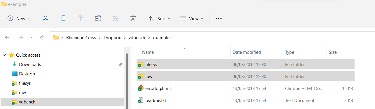
Example 1: Single run, one raw disk
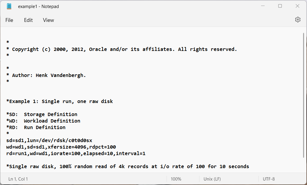
Example 2: Single run, two raw disk, two workloads.
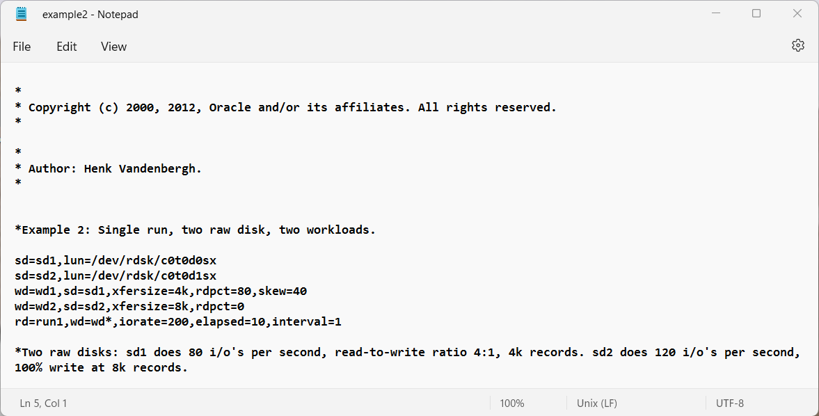
Example 3: Two runs, two concatenated raw disks, two workloads.
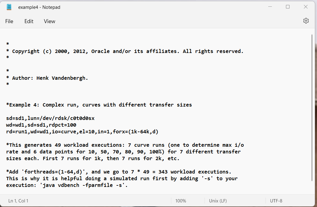
Example 4: Complex run, including curves with different transfer sizes
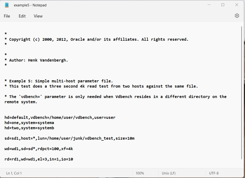
Example 5: Multi-host.
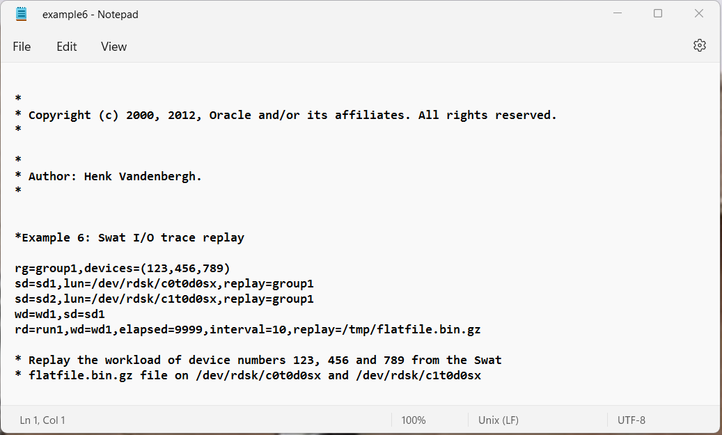
Example 6: Swat trace replay.
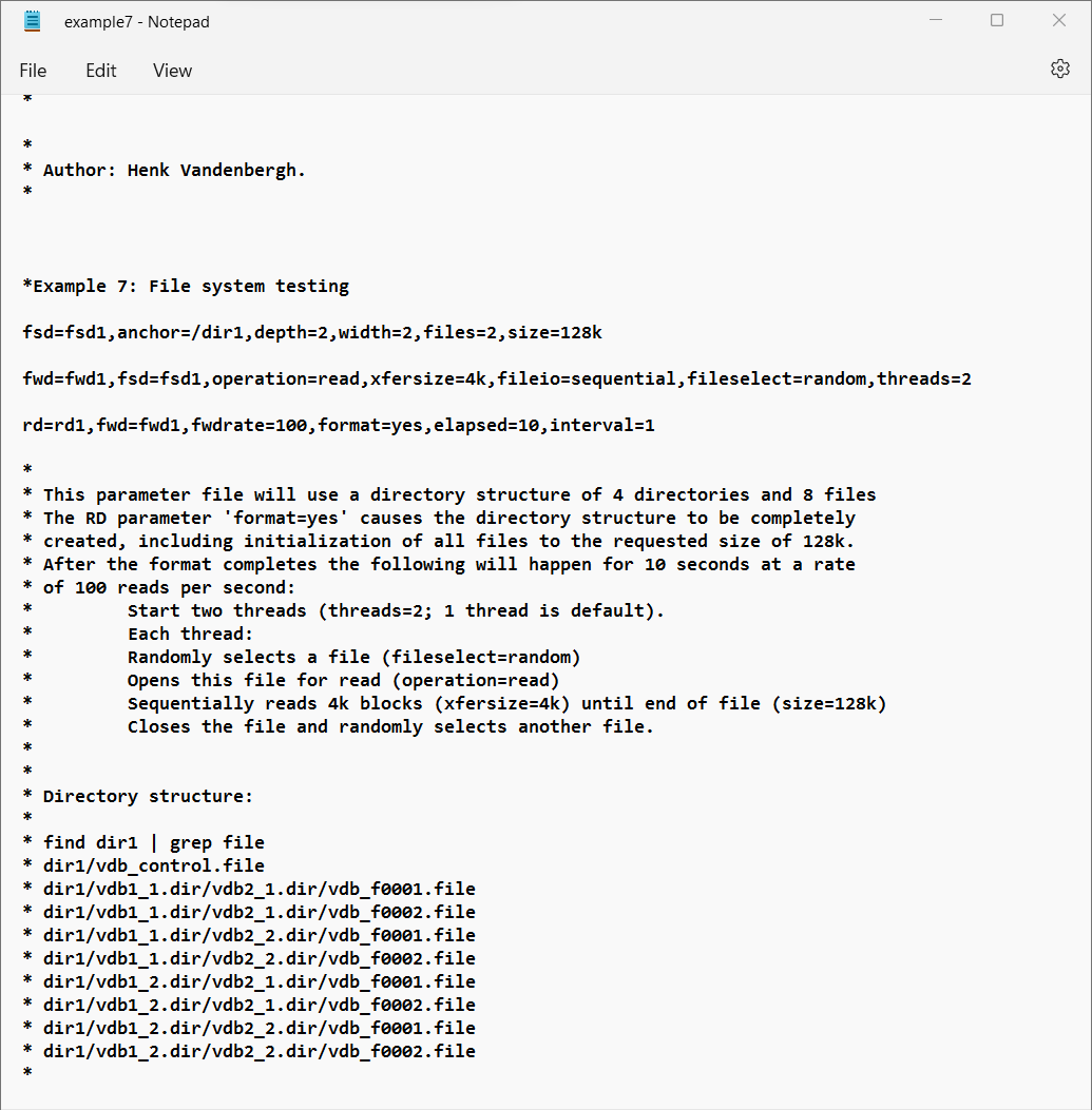
Example 7: File system test. See also Sample parameter file:
There is a larger set of sample parameter files in the /examples/ directory inside your Vdbench install directory inside the filesys and raw folders
Example 1
Example 2Example 3Example 4Example 5Example 6Example 7
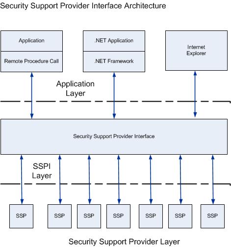
Alongside its operating systems, Microsoft offers the Security Support Provider Interface (SSPI) which is the foundation for Windows authentication. The SSPI provides a universal, industry-standard interface for secure distributed applications. SSPI is the implementation of the Generic Security Service API (GSSAPI) in Windows Server operating systems. For more information about GSSAPI, see RFC 2743 and RFC 2744 in the IETF RFC Database.
SSPI is a software interface. Distributed programming libraries such as RPC can use it for authenticated communications. Software modules called SSPs provide the actual authentication capabilities. The default Security Support Providers (SSPs) that invoke specific authentication protocols in Windows are incorporated into the SSPI as DLLs. An SSP provides one or more security packages
Security Support ProviderInterface Architecture
The SSPI in Windows provides a mechanism that carries authentication tokens over the existing communication channel between the client computer and the server. When two computers or devices need to be authenticated so that they can communicate securely, the requests for authentication are routed to the SSPI, which completes the authentication process, irrespective of the network protocol currently in use. The SSPI returns transparent binary large objects. These are passed between the applications, at which point they can be passed to the SSPI layer. The SSPI enables an application to use various security models available on a computer or network without changing the interface to the security system.
Security Support Provider
The following sections show the default SSPs that interact with the SSPI. The SSPs are used in different ways in Windows operating systems to enable secure communication in an unsecure network environment. The protocols used by these providers enable authentication of users, computers, and services; the authentication process, in turn, enables authorized users and services to access resources in a secure manner.
Using SSPI ensures that no matter which SSP you select, your application accesses the authentication features in a uniform manner. This capability provides your application greater independence from the implementation of the network than was available in the past.
Distributed applications communicate through the RPC interface. The RPC software in turn, accesses the authentication features of an SSP through the SSPI.
It’s been a while since I’ve blogged and in the interest of keeping a focus on training on new concepts, a friend suggested I follow John Zelle’s book- Python Programming – An introduction to Computer Science. The book is focused on Python but also provides some great detail on Computer Science principles along side programming.
As a result of having to do more programming at work, I thought I would chart my progress and register for a github account and document the end of chapter discussions, questions and exercises whilst learning some git concepts also
GitHub is a code hosting platform for version control and collaboration. It lets you and others work together on projects from anywhere. It has plenty of tutorials which can teach you GitHub essentials like repositories, branches, commits, and pull requests.
I have found it useful to my learning to document what I have learned, probably a repetitive learning concept and hopefully useful to others as it will be a public repository. If anyone feels like correcting anything or providing simpler and easier solutions, then feel free 🙂
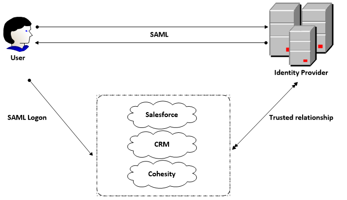
SAML is an XML-based open-standard for transferring identity data between two parties: an identity provider and a service provider. SAML enables Single-Sign On (SSO), a term that means users can log in once, and those same credentials can be reused to log into other service providers. The OASIS Consortium approved SAML v2 in 2005. SAML 2.0 changed significantly from 1.1 and the versions are incompatible.
What is XML used for in relation to SAML?
SAML transactions use Extensible Markup Language (XML) to communicate between the identity provider and service providers. SAML is the link between the authentication of a user’s identity and the authorization to use a service.
How does authentication and authorization work in SAML?
SAML implements a secure method of transferring user authentications and authorizations between the identity provider and service providers. When a user logs into a SAML enabled application, the service provider requests authorization from the appropriate identity provider. The identity provider authenticates the user’s credentials and then returns the authorization for the user to the service provider, and the user is now able to use the application.
SAML authentication is the process of checking the user’s identity and credentials. SAML authorization tells the service provider what access to grant the authenticated user.
What is a SAML provider?
There are two primary types of SAML providers, serviceprovider, and identity provider.
The identity provider carries out the authentication and passes the user’s identity and authorization level to the service provider.
A service provider needs the authentication from the identity provider to grant authorization to the user.
Advantages of SAML
Users only need to sign in once to access several service providers. This means a faster authentication process and the user does not need to remember multiple login credentials for every application.
SAML provides a single point of authentication
SAML doesn’t require user information to be maintained and synchronized between directories.
Identity management best practices require user accounts to be both limited to only the resources the user needs to do their job and to be audited and managed centrally. Using an SSO solution will allow you to disable accounts and remove access to resources simultaneously when needed.
Visualising SAML
SAML Example
SAML uses a claims-based authentication workflow. When a user tries to access an application or site, the service provider asks the identity provider to authenticate the user. Then, the service provider uses the SAML assertion issued by the identity provider to grant the user access.
The user opens a browser and navigates to the service provider’s web application, which uses an identity provider for authentication.
The web application responds with a SAML request.
The browser passes the SAML request to the identity provider.
The identity provider parses the SAML request.
The identity provider authenticates the user by prompting for a username and password or some other authentication factor. NOTE: The identity provider will skip this step if the user is already authenticated.
The identity provider generates the SAML response and returns it to the user’s browser.
The browser sends the generated SAML response to the service provider’s web application which verifies it.
If the verification succeeds, the web application grants the user access.
We had an interesting problem with a 6 host vSAN cluster where 1 host seemed to be in a network partition according to Skyline Health. I thought it would be useful to document our troubleshooting steps as it can come in useful. Our problem wasn’t one of the usual network mis-configurations but in order to reach that conclusion we needed to perform some usual tests
We had removed this host from the vSAN cluster, the HA cluster and removed from the inventory and rebuilt it, then tried adding it back into the vSAN cluster with the other 5 hosts. It let us add the host to the current vSAN Sub-cluster UUID but then partitioned itself from the other 5 hosts.
Usual restart of hostd, vpxa, clomd and vsanmgmtd did not help.
Test 1 – Check each host’s vSAN details
Running the command below will tell you a lot of information on the problem host, in our case techlabesxi1
Straightaway we can see it is partitioned as the Sub-Cluster Member UUIDs should have the other 5 hosts’ UUID in and the Sub-Cluster Member Hostnames should have techlabesxi2, techlabesxi3, techlabesxi4, techlabesxi5, techlabesxi6. It has also made itself a MASTER where as we already have a master with the other partitioned vSAN cluster and there can’t be two masters in a cluster.
Master role:
A cluster should have only one host with the Master role. More than a single host with the Master role indicates a problem
The host with the Master role receives all CMMDS updates from all hosts in the cluster
Backup role:
The host with the Backup role assumes the Master role if the current Master fails
Normally, only one host has the Backup role
Agent role:
Hosts with the Agent role are members of the cluster
Hosts with the Agent role can assume the Backup role or the Master role as circumstances change
In clusters of four or more hosts, more than one host has the Agent role
Test 2 – Can each host ping the other one?
A lot of problems can be caused by the misconfiguration of the vsan vmkernel and/or other vmkernel ports however, this was not our issue. It is worth double checking everything though. IP addresses across the specific vmkernel ports must be in the same subnet.
Get the networking details from each host by using the below command. This will give you the full vmkernel networking details including the IP address, Subnet Mask, Gateway and Broadcast
esxcli network ip interface ipv4 address list
It may be necessary to test VMkernel network connectivity between ESXi hosts in your environment. From the problem host, we tried pinging the other hosts management network.
vmkping -I vmkX x.x.x.x
Where x.x.x.x is the hostname or IP address of the server that you want to ping and vmkX is the vmkernel interface to ping out of.
This was all successful
Test 3 – Check the unicast agent list and check the NodeUUIDs on each host
To get a check on what each host’s nodeUUID is, you can run
esxcli vsan cluster unicastagent list
Conclusion
We think what happened was that the non partitioned hosts had a reference to an old UUID for techlabesx01 due to us rebuilding the host. The host was removed from the vSAN cluster and the HA cluster and completely rebuilt. However, when we removed this host originally, the other hosts did not seem to update themselves once it had gone. So when we tried to add it back in, the other hosts didn’t recognise it.
The Fix
What we had to do was disable ClustermemberListUpdates on each host
Don't think about what can happen in a month. Don't think what can happen in a year. Just focus on the 24 hours in front of you and do what you can to get closer to where you want to be :-)